Robert A McDougal

XPPAUT is a program by Bard Ermentrout of the University of Pittsburgh for solving a variety of dynamical systems problems on the computer. His official tutorial is located here, but we will only concern ourselves with the basics.

Outline of Contents

• Plotting Solutions to Ordinary Differential Equations
  • A Simple, First Order ODE
  • Changing the Window
  • Setting the Initial Conditions
  • Saving Images as Postscript Files
  • Displaying Numerical Values of Solution
  • A Second Order ODE
  • Converting a High Order ODE to a First Order System
  • Change Variables Plotted
  • Add a Curve to the Graph
  • PIR in Mutually Coupled FitzHugh-Nagumo Neurons
  • Parameters
  • Functions
  • Logical Expressions and Split Functions
  • Arrays
  • Configuring XPPAUT from the .ODE File
• Delay Equations
  • Auxillary Functions
• Phase Planes
  • Use the Mouse to Select Initial Conditions
  • Flow
  • Nullclines
  • Fixed Points
• Bifurcation Diagrams

Plotting Solutions to Ordinary Differential Equations

A Simple, First Order ODE

We start by concerning ourselves with one of the simplest Initial Value Problems that we can think of,

This problem clearly has solution x(t) = −1 + t. We graph it with XPPAUT. First, let's create a text file sample1.ode:

# sample1.ode
# Solves the initial value problem dx/dt=1, x(0)=-1
dx/dt=1
x(0)=-1
done

The first two lines are comments and are ignored by XPP. In the third line, we specify the differential equation. The fourth line gives the initial value condition, and the fifth line tells XPP that we are done stating the system.

Warning: Do not be deceived by the statement x(0)=-1. You cannot say x(1)=-1 if you instead wanted to start integrating from t = 0. The general way to state initial conditions is to use the form init x=-1 or just i x=-1.

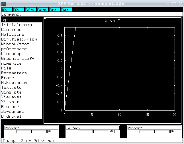
We have the computer solve our ODE by typing xppaut sample1.ode at the command line. A window appears:

Click Initialconds and then (O)ld to plot using the initial conditions we specified in the .ode file. (Note: In XPPAUT, you can also just type the capitalized letter in a menu choice instead of clicking it. In our case then, we would just type io to graph.)

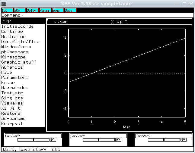
We have a graph, but the axes need adjusting. Click Viewaxes, then 2D to display the axes menu.

Here we can specify which variables we want to plot, the range of x and y values, and labels for the axes. In the image above, I have changed the y values to run from −5 to 5 and the x values to run from 0 to 5. I also put labels on the axes.

To change the initial condition, click on the cyan colored button ICs in the upper left-hand corner. A new window appears.

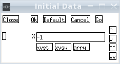
Change your initial condition and click Go. A new line is drawn on your graph. To clear the graph before drawing a new trajectory, click Erase (or type e) before clicking Go. I for example chose to add a trajectory starting with x = −3.

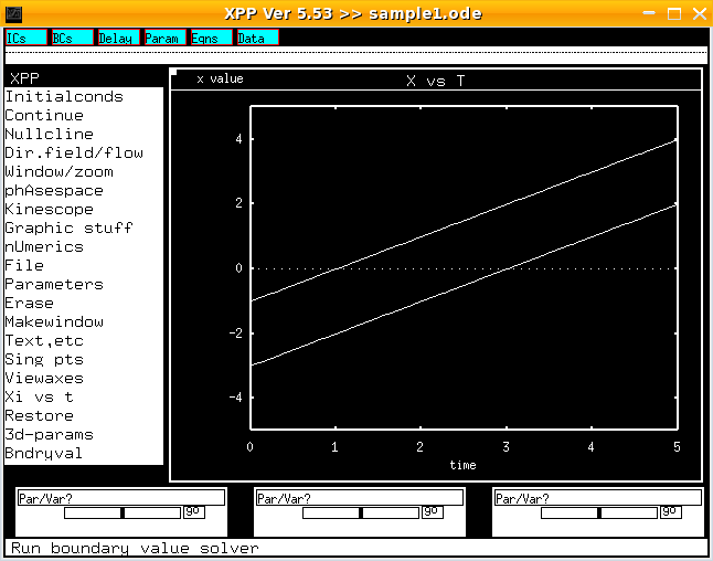
Warning: It is important to note that XPPAUT only stores your graph data if you explicitly tell it to by selecting Graphic stuff and then (F)reeze, which stores the last trajectory plotted. If you do not make that selection, the old trajectory will be erased if the window is redrawn, it will not be saved if you try to save the image, etc...

To save our trajectories as a postscript file, select Graphic stuff and then (P)ostscript. For now, hit Ok on the Postscript Parameters window, enter a filename and then click Ok to save.

Plotting trajectories can help you get an intuitive sense of what is going on, but in many situations you want to know specific function values, either for their own sake or so you can do further analysis on the problem in another program. To do so, click on the cyan colored button Data and a new window will appear.

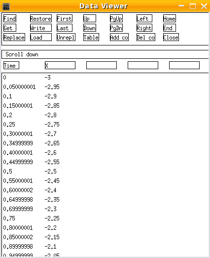
Note that the time values are spaced every $.05$. This is the default. To change this behavior, select nUmerics and then Dt. Options for scrolling and writing the data to disc are available at the top of the window.

A Second Order ODE

Consider the ODE

which has solution x(t) = sin(t). XPPAUT only works with first order equations or systems of equations, not second order. Fortunately by making the change of variables

we can turn any second order ODE into a system of two first order ODEs. Similarly, any higher order ODE can also be reduced to a system of first order ODEs. In our case, for example, the system becomes:

Our system then has solution x(t) = x₁(t) = sin(t) and x₂(t) = cos(t). We enter the problem into XPPAUT as sample2.ode:

# sample2.ode
# solves the system form of x''=-x, x(0)=0, x'(0)=1
dx1/dt=x2
dx2/dt=-x1
x1(0)=0
x2(0)=1
done

As before, we run it by typing xppaut sample2.ode at the command prompt, clicking on the cyan button ICs and selecting Go. We then have the following window.

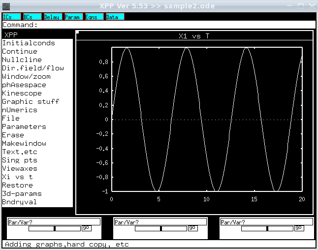
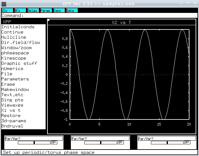
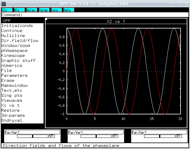
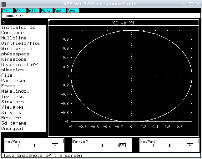
Note that it plotted X1 vs t. To see X2 vs t instead, select Viewaxes then 2D and change Y-axis to X2. (We could even plot X1 vs X2 -- which in our case would give us a circle. See the Phase Plane section for more.)

Click Ok and the sine wave should be replaced with a cosine wave.

We may prefer to have both X1 and X2 plotted at the same time. For example, in a later example we consider the interactions of two mutually coupled neurons, and we would like to see both of their electrical outputs simultaneously. Fortunately, XPPAUT gives us an easy way to add a curve to the current graph. Select Graphic stuff, then (A)dd curve; a new dialog box appears.

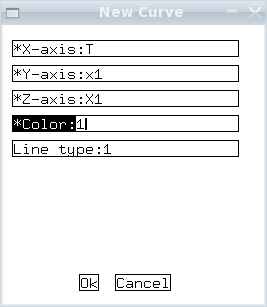
Here I have changed Y-axis to x1 (case does not matter in XPPAUT) and Color to 1. (The Z-axis option does not matter since we are only working with a two-dimensional image.) Click Ok and the curve will be added. (The new curve will be red since we set Color to 1; other color choices are available.)

PIR in Mutually Coupled FitzHugh-Nagumo Neurons

We now attempt sample3.ode, a more complicated example that introduces a number of new concepts.

# sample3.ode
# Post Inhibitory rebound in mutually coupled
# FitzHugh-Nagumo cells.

# gsyn=2 gives suppressed, gsyn=.5 gives pir

# Parameter values. It's always better to give constants
# as parameters so you can change them without exiting
# XPP.
p vSpike=-1, eps=.2, gsyn=.5, theta=-.2,scale=10
p wshift=3.8, vshift=0, scale2=10
p alpha=1, beta=.1, vstart=0, wstart=0, vsyn=-2

# Usually we talk of the FitzHugh-Nagumo model with
# f and g somewhat arbitrary, but to do numerics we
# need to pick specific functions.
f(a,b)=-b-15*(a-1)*a*(a+1)
g(a,b)=-b+scale*tanh(a*scale2)+wshift

# the slow system (equation) and the synapse obey
# the same rules for both neurons, so we use this array
# notation. The first line denotes the range of j (always
# j) and v[j] denotes the j'th v value, etc...
%[1..2]
w[j]'=eps*g(v[j],w[j])
s[j]'=alpha*(1-s[j])*(v[j]>theta)-beta*s[j]
%

# cell 1 receives input from 2 and 2 from 1, so we write
# these seperately since they are different
v1'=f(v1,w1)-gsyn*(v1-vsyn)*s2
v2'=f(v2,w2)-gsyn*(v2-vsyn)*s1

# initial conditions. Since I don't specify s values,
# they start at 0.
i v1=0, w1=-5, v2=-1, w2=-2

# configure XPP's options.
@ total=100, xlo=0, xhi=100, ylo=-1.5, yhi=1.5
@ nplot=2, xp[1..2]=t, yp[j]=v[j]
done

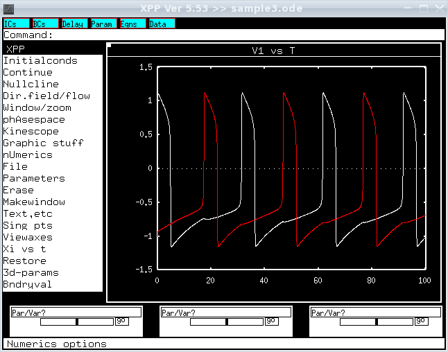
Integrating using the default settings gives us the following graph. Note how the membrane potential of each neuron drops a little when the other is firing; the drop is because the neurons inhibit each other.

Parameters

Sometimes our system is critically dependent on the particular numbers in our equations. (Bifurcation diagrams help us understand this dependency.) When you first attempt to model a problem, you may not know the constants. Using parameters (the lines beginning with the letter p) we can change the constants within XPPAUT, by simply clicking on the cyan colored button labelled Param.

Exercise. Vary the parameters to see what other behaviors you can get out of the system. Can you make the neurons fire together? Can you make it so that only one neuron is firing?

Functions

Notice the lines

f(a,b)=-b-15*(a-1)*a*(a+1)
g(a,b)=-b+scale*tanh(a*scale2)+wshift

They define two functions, f and g, that I can use elsewhere in my code. The ability to define functions helps with readablility and maintainability of your .ODE files.

Logical Expressions and Split Functions

As a first approximation, a synapse only experiences a buildup of neurotransmitters when the membrane potential of the presynaptic cell is above a certain threshold, in our case theta. Fortunately, logical expressions return 1 if they are true, 0 if false. That is, (2>1) returns 1, (2<1) returns 0, or more interestingly (v>theta) returns 1 whenever v is bigger than theta. This allows us to construct split functions by multiplying the logical expression by its corresponding value and adding all such values together.

Arrays

SAY SOMETHING HERE???

Controlling XPPAUT from the .ODE File

Lines beginning with @ configure XPPAUT's initial settings. xlo, xhi, ylo, and yhi are probably the most useful settings as they let you set the initial window. dt requests a step size; the default is .05. total sets the length of time to integrate over; the default is 20. SAY MORE???

Exercise: Implement a Hodgkin-Huxley neuron with a constant applied current term as a parameter. Initially, m = m_∞(V_rest), h = h_∞(V_rest), and n = n_∞(V_rest). With an applied current of 0, show that your neuron will not fire if it starts with a membrane potential near rest but that it will fire if the initial membrane potential is sufficiently above or below rest. Next, start with the membrane potential at rest and increase the applied current. What happens?

Delay Equations

Synapses and other biological processes often act after a delay. A detailed model might explain this delay by some set of chemical reactions, but often only the delay is relevant. XPPAUT lets us incorporate a delay with the function delay. For example, delay(x,3) returns the value of x at a time of 3 before the current time. You also must set the @delay setting to an amount bigger than your longest delay.

In sample3, for example, we represented the delay due to the build up and decay of neurotransmitters in the synapses by using a differential equation for the synapse. Unfortunately, this gives us a differential equation for each synapse. As a cruder approximation, we can instead model a synapse as either on or off, switching after a delay of tau. This is sample4.ode:

# sample4.ode
# Post Inhibitory rebound in mutually coupled
# Fitzhugh-Nagumo cells; delay equation version.

# Parameter values. It's always better to give constants
# as parameters so you can change them without exiting
# XPP.
p vSpike=-1, eps=.2, gsyn=.5, theta=-.2,scale=10
p wshift=3.8, vshift=0, scale2=10
p tau=2, vsyn=-2

# Usually we talk of the FitzHugh-Nagumo model with
# f and g somewhat arbitrary, but to do numerics we
# need to pick specific functions.
f(a,b)=-b-15*(a-1)*a*(a+1)
g(a,b)=-b+scale*tanh(a*scale2)+wshift

# the slow system (equation) and the synapse obey
# the same rules for both neurons, so we use this array
# notation. The first line denotes the range of j (always
# j) and v[j] denotes the j'th v value, etc...
%[1..2]
w[j]'=eps*g(v[j],w[j])
s[j]=delay(v[j],tau)>theta
aux syn[j]=s[j]
%

# cell 1 receives input from 2 and 2 from 1, so we write
# these seperately since they are different
v1'=f(v1,w1)-gsyn*(v1-vsyn)*s2
v2'=f(v2,w2)-gsyn*(v2-vsyn)*s1

# initial conditions. Since I don't specify s values,
# they start at 0.
i v1=0, w1=-5, v2=-1, w2=-2

# configure XPP's options.
# delay=10 means that we must use a delay of less than 10
@ total=100, xlo=0, xhi=100, ylo=-1.5, yhi=1.5
@ delay=10
@ nplot=2, xp[1..2]=t, yp[j]=v[j]
done

Graphing it in XPPAUT using the default settings gives us:

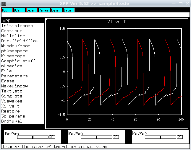
Note that the inhibition of a neuron happens a time of tau=2 after the other one begins to fire and is released tau=2 after the membrane potential of the other neuron drops.

Auxillary Functions

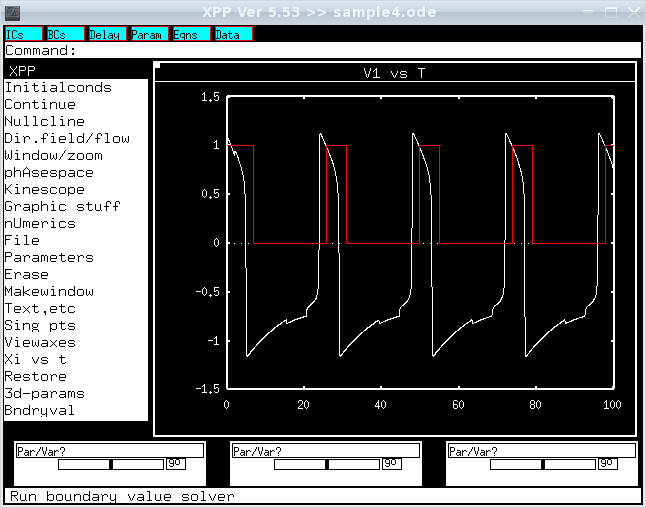
Functions, in the sense described previously, cannot be graphed directly. Instead, we must create an auxillary function, as in the following:

aux syn[j]=s[j]

Recall that in our example, s[j] was a function. This line lets us plot synaptic levels just as we could (but did not) when we looked at sample3. Here, I plot both v1 (white) and syn1 (red) as functions of time.

Phase Planes

Let us return to our second ODE:

We now plot X2 vs X1.

Use the Mouse to Select Initial Conditions

Select Initialconds then either (M)ouse to select one initial condition by clicking with the mouse or m(I)ce to repeatedly select initial conditions and plot trajectories. SAY MORE???

Flow

Rather than click over and over again, you can select Dir.field/flow and then (F)low to see the trajectories starting at evenly spaced grid points in phase space. (You are prompted for grid spacing at the top of the main window; simply press enter to select the default values.) SAY MORE???

Nullclines

Plot Nullclines by selecting Nullcline and then (N)ew. Remember fixed points of a two-dimensional system are precisely those points where the nullclines intersect. SAY MORE???

Fixed Points

Points where the derivatives are all 0 are called fixed points; they may be stable, unstable, or nodes. To locate the fixed points exactly, use Sing pts. In our simple example, we can just click (G)o after that. Select Yes when asked if you want to print the eigenvalues (they will appear in your terminal window). A new window then appears with information about the fixed point it found. In our case, there is only one, but in general you may have to use one of the other options in the Equilibria menu to find other fixed points.

SAY MORE???

Exercise. Open sample3 in XPPAUT. Set gsyn to 0 to decouple the neurons. Select Graphic stuff then (D)elete last to go back to just drawing one plot (and hence one neuron's output). Graph W1 vs V1. What happens as you vary wshift? How does that affect the nullclines? The flow? Can you describe the role of eps?

Bifurcation Diagrams

The "AUT" in XPPAUT refers to AUTO, a program for drawing bifurcation diagrams for ODEs which is included with XPP. SAY MORE???